Summary
Dynamical Systems Approaches to Infectious Disease Epidemiology/Ecology/Evolution (DSAIDE) is an R package that allows you to explore and study concepts of infectious disease epidemiology (ecology/evolution) using dynamical systems models.
The main way of interaction with the models is through a graphical user interface. It is not necessary - though possible - to read or write computer code.
The package also provides a path toward using and building your own models by relatively seamlessly moving from the graphical user interface to direct interaction with pre-written simulations all the way to modifying the underlying simulations to fit your needs.
The different use cases for the package are described below.
Package description
The package consists of several simulations (referred to as apps)
that allow for the simulation and exploration of different topics
related to infectious disease dynamics. The underlying models are
written as compartmental simulation models, either deterministic using
differential equations (deSolve package) or stochastic
using a Gillespie-type approach (adaptivetau package). A
graphical user interface is wrapped around each simulation/app. The
graphical user interface is written using the functionality of the R
shiny package. This allows exploration of models and
concepts without the need to write any code. At the same time, the
package is structured in a way that should allow those interested in the
actual models and learning R coding to easily move from one stage to
another.
Each app is meant to be fully self-explanatory and contains a description of the model, a list of tasks the user could try, and further information on background reading and other resources.
Intended audience and goal of the package
The package is geared towards individuals who want to learn how simulation models are used to study and understand infectious disease epidemiology/ecology/evolution. The package teaches concepts such as patterns of infectious disease incidence, the reproductive number, extinctions and critical community size, and more. All these concepts are not well described by applying classical epidemiology approaches (i.e. assuming independence between individuals), but can readily by understood using a systems/modeling approach.
While I originally wrote the package as a component of a course on infectious disease epidemiology/modeling, the documentation for each app tries to be fairly complete and self-contained. This should allow you to get some understanding of the topics and models without requiring additional information. If you use this package on your own without taking a class on the topic, it might be possible to fully learn the material covered by the apps by working through the Tasks for each app and filling any gaps with some of the references provided for each app (see the Further Information section for each app) or by consulting some general infectious disease modeling textbooks, e.g. (Keeling and Rohani 2008; Vynnycky and White 2010; Bjørnstad 2018) or my online textbook or course materials.
Pre-requisites
Since DSAIDE is an R package, you need to
have R installed. I also
recommend RStudio, though
it’s not required. If you are not familiar with R you can
find a
brief introduction here, which also provides pointers to detailed
install instructions.
Installation
After having installed and opened R/Rstudio, you can install the package from CRAN by typing the following into the R console (the bottom left window if you are using RStudio):
install.packages('DSAIDE')Alternatively, you can install the latest development version (with
usually both more features and more bugs) from github, using the
remotes package. The following commands, typed into the
R console, will get you up and running:
install.packages('remotes') #if not already installed
remotes::install_github('ahgroup/DSAIDE')
The package depends on other packages, which will also be installed
as needed. Package installation is a one-time process, unless you update
or re-install R itself, or want to install a newer version of
DSAIDE.
Using the package
The following sections describe the main envisioned ways the content in this R package can be used and extended. The idea is that you start at level 1, and then depending on needs and interests, you can decide to move on to the next level.
Level 1: Interactive use through the graphical user interface
The interactive exploration of the models and infectious disease concepts through the graphical user interface is the main intended use of this package. The steps to get there are simple.
Load and run the package
After install, load the package by typing the following into the
R console.
You need to load the package every time you start a new R/Rstudio session.
If the package loads correctly, you should receive a short greeting.
Now you can open the main menu by typing the following into the
R console:
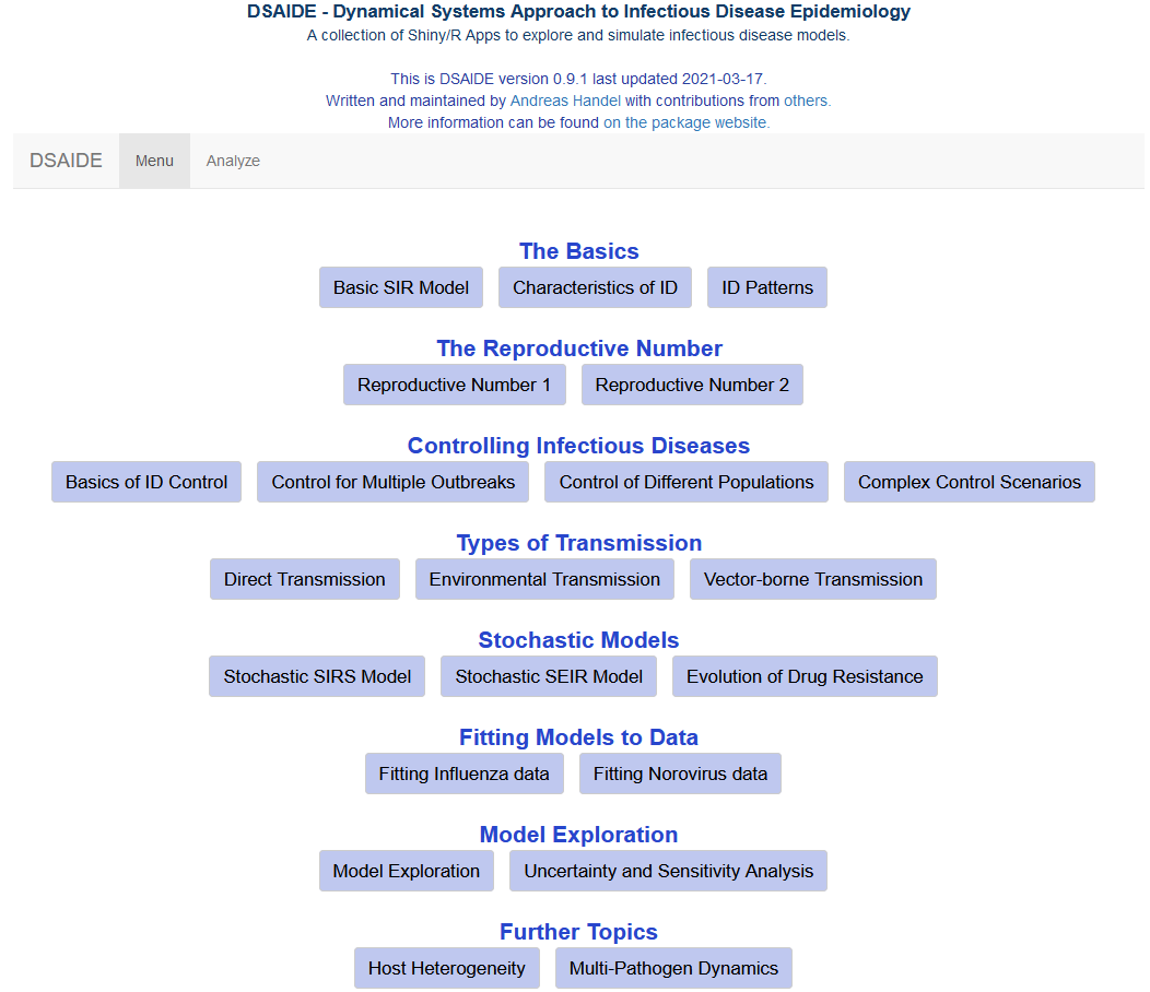
If successful, you should see a graphical menu open in your browser that looks similar to this (looks might differ a bit depending on the version of DSAIDE you are running):

Main menu of the DSAIDE package.
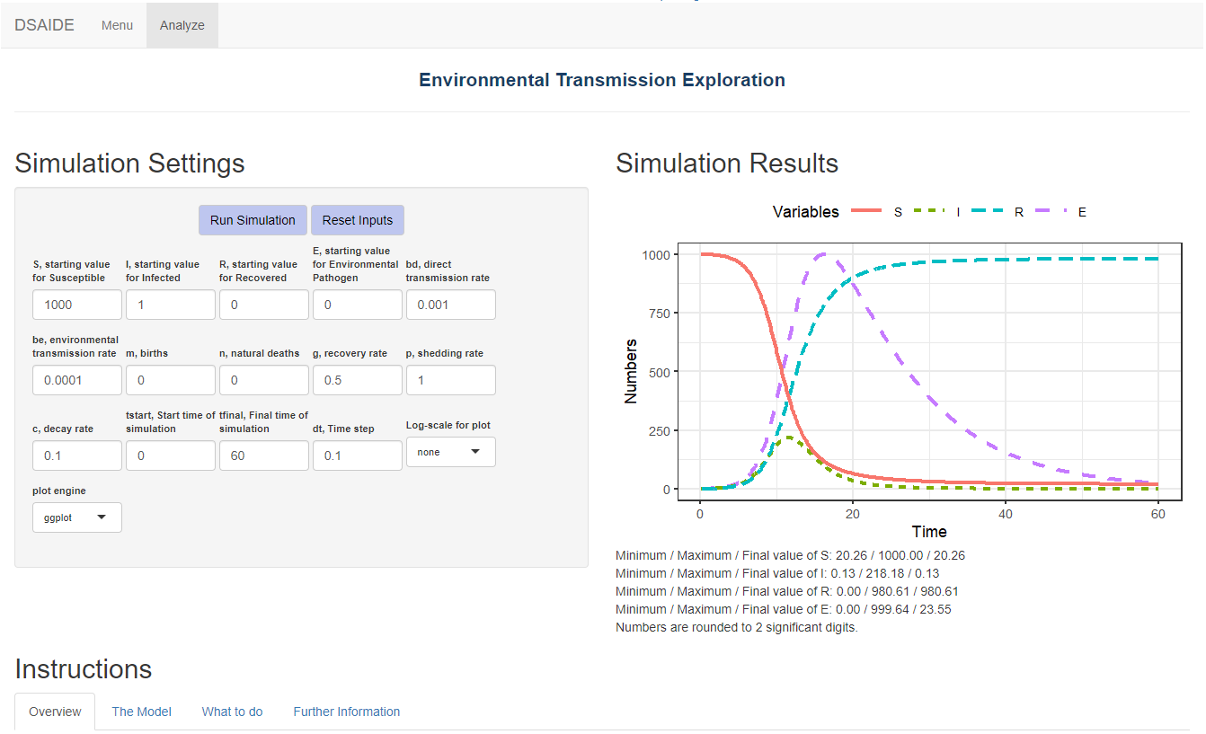
From the main menu, you can choose the different apps corresponding to different topics. Each app has the model inputs you can set on the left and the outputs (figures and text) on the right. This is an example of one of the apps:

Screenshot of the input-output elements of one of the apps.
As seen in the figure above, below each app are four tabs with different sections providing information and instruction.
The Overview tab provides a brief overview, introduction and list of learning objectives.
The Further Information tab tells you the name(s) of the underlying models and often provides references to resources (books and papers) on that topic.
The two most important tabs are the Model and What to do tabs.
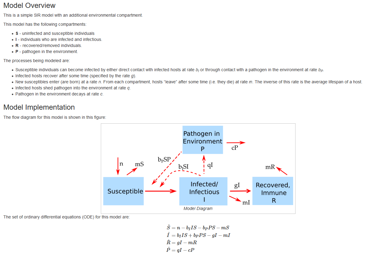
The Model tab gives a detailed description of the model underlying the app, shows the model diagram and equations, and provides any other further information needed to understand what is going on. The following figure shows an example of this for one of the apps.

Screenshot of the Model section of one of the apps.
To use the package, you do not need to do any math with differential equations, i.e. no calculus (you will have to do a bit of algebra for some tasks.) By seeing the model equations, diagram and description, you should be able to learn how these models are set up and what the different model terms mean and do. The idea is that you learn how to read those models (and if inclined, build and implement your own, see below), but you will not need to do any complicated math involving differential equations.
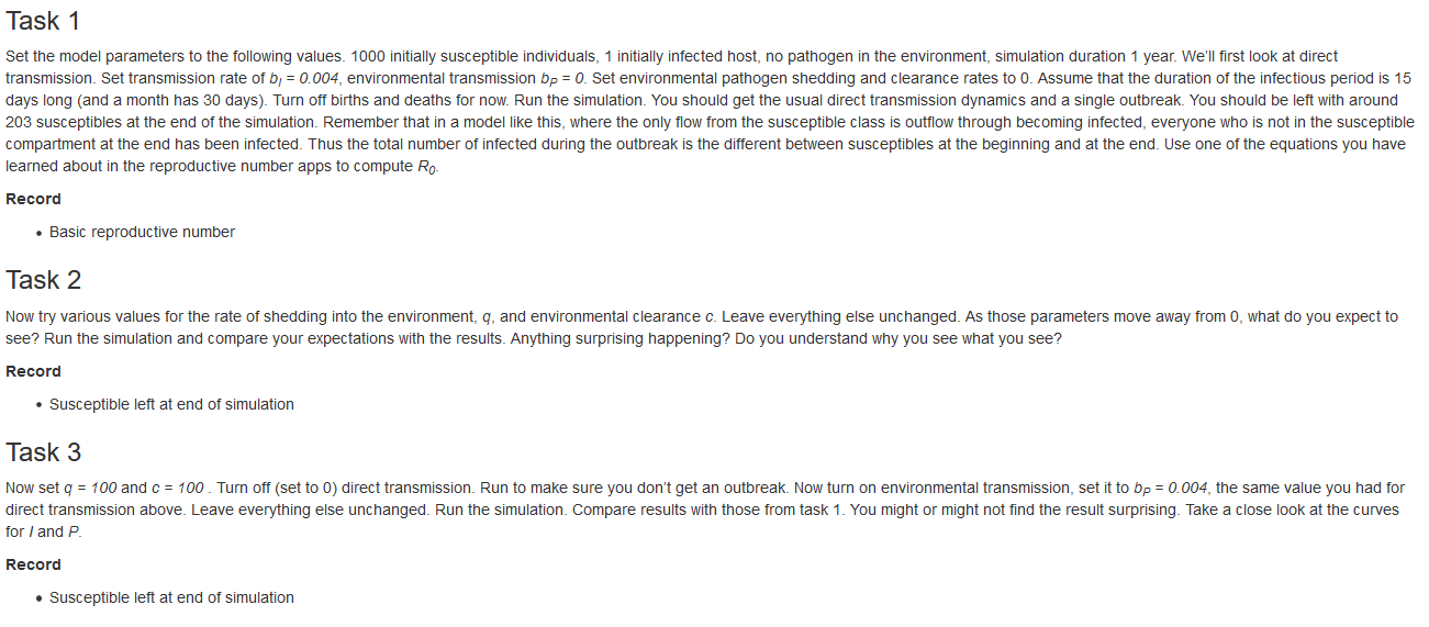
The What to do tab contains a list of suggested tasks you might want to go through. By doing those tasks, you will learn the topic a specific app is meant to teach. The following figure shows an example for part of one of those What to do sections.

Screenshot of the What to do section of one of the apps.
For learning the material and topic, going through all the tasks in
the What to do section is the most important part. The idea is
that by working through the tasks you will be able to learn the topic
the app is meant to teach. If you are using the package as part of a
course, you might be asked to write down and submit the answers you are
asked to record for each task. Once you finished exploring a specific
app, you can return to the main menu by clicking the Menu
button in the upper left corner.
The apps are arranged in roughly the order you should go through
them. You should definitely start with all apps in
The Basics section, even if you are already familiar with
some of these models, since those apps introduce some general ideas and
conventions that are specific to DSAIDE. In general, at the beginning of
an app there will be information telling you which other apps are
assumed as pre-requisite knowledge.
Once you are done exploring DSAIDE, you can exit back to the
R console by clicking the Exit button.
Level 2: Directly interacting with the simulation functions
Using DSAIDE through the Level 1 approach just described means you will not need to read or write any code. If an when you want to learn more, you can proceed to Level 2.
Once you are comfortable interacting with the models and have a good understanding of the concepts covered by the different apps, it is possible, without too much effort, to interact with the simulation models directly. This provides more flexibility at the cost of writing a limited amount of code.
To facilitate direct interaction and modification of the underlying simulations, each app is structured in such a way that the underlying model/simulation is a stand-alone function. For some apps, there are multiple underlying functions involved. Assuming you have loaded the package, you can call any of these functions directly, without going through the graphical interface. The Further Information tab inside each app provides the name of the corresponding underlying function(s) and how to call their help files to get information on their use.
Consider as example the first app, Basic SIR Model. As you
can read in the Further Information tab, this app uses two
simulator functions, simulate_SIR_model_ode and
simulate_SIR_model_discrete. After loading the package (if
not already loaded) with
## Loading required package: shiny## Welcome to the DSAIDE package. Type dsaidemenu() to get started.you can learn about the inputs and outputs of the model/function by
looking at its documentation. For instance for the first simulator
function, simulate_SIR_model_ode, you can type the
following into the R console:
help('simulate_SIR_model_ode')The help file explains that you can run the simulation by specifying initial number of individuals in each compartment (susceptible, infected, recovered), the parameters governing the model processes (here the rates of infection and recovery), as well as time parameters (start time, end time, and time step). Note that the time step determines the times for which results are returned, not the internal time step during simulation.
Each parameter has some default, listed in the help file. Running a simulation model without any specifications runs it with the defaults:
result <- simulate_SIR_model_ode()Calling the simulation function runs the underlying model (here a simple 3 compartment ODE model, as described in the Model section of the app). Most simulation functions produce and return time-series for the dynamics of each of the variables that are tracked as a list. What exactly is returned is described in the help file for each function.
You can take the results returned from the simulation function and further process them. For instance you could plot the time-series for susceptible as function of time:
plot(result$ts[ , "time"],result$ts[ , "S"],xlab='Time',ylab='Number Susceptible',type='l')
You can overwrite the default settings by providing your own values for specific parameters, as shown in this example:
result <- simulate_SIR_model_ode(S = 2000, b = 0.001, g = 0.5, tfinal = 200)
plot(result$ts[ , "time"],result$ts[ , "S"],xlab='Time',ylab='Number Susceptible',type='l')
Any values that you do not specify will be kept at their defaults.
Note that unless explicitly specified, the models do not have inherent time units. Instead, those depend on the time units you choose for the parameters. It is important to ensure that all quantities (parameters and time settings) have the same time units, e.g. days or months (or the inverse of those units for the rate parameters).
Not all simulator functions return time-series. For instance the function underlying the uncertainty and sensitivity app returns specific outcomes (maximum and final state of variables) for different parameter values. In every instance, the documentation for the function explains what is returned, so you know how to take the returned results and further process them.
The ability to call the simulation functions directly instead of going through the graphical interface allows additional exploration of the models. For instance if you wanted to explore the behavior of a model systematically for different values of a given parameter, this would need to be done manually if run through the graphical interface. Calling the function directly allows you to automate this by wrapping the function inside a loop over the parameter of interest, recording some quantity of interest for each run, and report the result at the end. The following is a simple example, showing a loop over different values of the recovery rate and recording the peak of the outbreak each time, with the final result peak of outbreak as function of recovery time shown in a plot:
gvec = seq(0.01,0.3,by=0.01) #values of recovery rate, g, for which to run the simulation
peak = rep(0,length(gvec)) #this will record the peak values for each g
for (n in 1:length(gvec))
{
  #call the simulator function with different values of g each time
  result <- simulate_SIR_model_ode(S = 500, b = 1/2500, g = gvec[n],  tfinal = 200)
  peak[n] <- max(result$ts[,"I"]) #record max number of infected for each value of g
}
#plot final result
plot(gvec,peak,type='p',xlab='Rate of recovery',ylab='Max number of infected')
Thus, you can add your own custom code to the existing simulator functions and with a few lines of extra code analyze and explore many more questions and scenarios than those accessible through the graphical interface. This provides a lot more flexibility, but requires writing some R code to interface with the supplied simulator functions.
Level 3: Modifying the simulation functions
While level 2 provides the user with a fair amount of flexibility and
the ability to investigate the models and ask questions that would be
hard or impossible going through the graphical interface, there is still
one major constraint. Namely this approach only allows use and analysis
of pre-written, existing simulation models. This constraint can be
overcome by directly modifiying and customizing the underlying
simulation functions. As was true for moving from level 1 to 2, this
move from level 2 to what I call level 3 provides further (almost
unlimited) flexibility at the cost of having to write increasingly more
R code.
To make modifying the existing functions easy, copies of all
simulator functions are provided in a folder called
simulatorfunctions which can be downloaded as a zip file from
the main menu. Each function in that folder starts with
simulate_. The Further Information section in each
app tells you which simulator function goes with which app.
The code for each simulator function is (hopefully) well documented.
Some basic to intermediate level of R coding experience is
likely required to successfully modify the functions. In addition to
modifying the simulator function of interest, you will likely also have
to write some additional code to interact with their modified function
(as described in Level 2).
The following provides a simple example of this process of modifying
a simulator function and exploring its results. Assume that we want to
modify the simple SIR model encoded in simulate_sir_ode.R.
(To make things easy, the name of a .R file containing the
code and the name of the function itself are the same.) After finding
the file, making a copy and renaming it (called
mysimulator.R here), we can make modifications.
Say we want to include waning immunity with recovered returning to the susceptible class at rate w.
We will need to modify the following lines of code:
old:
simulate_SIR_model_ode <- function(S = 1000, I = 1, R = 0, b = 0.002, g = 1, tstart = 0, tfinal = 100, dt = 0.1) new:
mysimulator <- function( S = 1000, I = 1, R = 0, b = 0.002, g = 1, w = 0, tstart = 0, tfinal = 100, dt = 0.1 ) old:
parvec_mb = c(b = b, g = g) new:
parvec_mb = c(b = b, g = g, w = w)old (ignoring comments present in the code):
dS_mb = -b*S*I
dI_mb = b*S*I -g*I
dR_mb = g*I
new:
dS_mb = -b*S*I +w*R
dI_mb = b*S*I -g*I
dR_mb = g*I -w*R
Note that if we wanted to share this function with others, we would need to also update the function documentation at the start of the file. For personal use of the function, this is a good idea but not required.
We could now for instance explore how different rates of waning immunity impact the maximum peak size over all outbreaks. This requires a slight modification of the code shown above in Level 2 as follows:
source('mysimulator.R') #to initialize the new function - it needs to be in same directory as this code
wvec = seq(0,1,by=0.02) #values of immunity loss rate, w, for which to run the simulation
peak = rep(0,length(wvec)) #this will record the peak values for each g
for (n in 1:length(wvec))
{
  result <- mysimulator( S = 1000, I = 1, R = 0, b = 1e-3, g = 0.5, w = wvec[n], tstart = 0, tfinal = 300, dt = 0.1)
  peak[n] <- max(result$ts[,"I"])
}
plot(wvec,peak,type='p',xlab='Rate of waning immunity',ylab='Max number of infected')
For most users and especially novice coders, it is likely best to
start with one of the provided models and modify as needed. However, at
this level, you have essentially full control and are only limited by
what can be accomplished using the R programming language
and your ability and interest in writing customized code.
Contributing to the package
The package is on GitHub and you can use the usual GitHub process to file bug reports, send feature requests, contribute updates and bug fixes, etc. If you have any comments or feedback, I very much welcome them. Please file a GitHub issue and let me know what you think.
The package is built in a way that makes it (hopefully) easy for others to contribute new simulations/apps. To that end, the package contains this Markdown file which provides further information on the details of the package structure. If you plan to develop new apps, or make other substantial contributions, it’s best to get in touch with me first via email or GitHub.
Further information
See the package website for useful additional information.
Contributors
This R package is developed and maintained by Andreas Handel. A full list of contributors and a Bibtex entry for the citation can be found here.
Citation
If the package does in any way help you with your work such that it warrants citing in one of your papers, please cite this publication in PLoS Computational Biology.